Show code for vector generation
# Generate a sample vector
sample_vector <- c(rep(10, 50), rep(20, 25), rep(30, 20), rep(40, 5), rep(3, 200), 1000)In this practical we are going to implement the various techniques discussed in the section Data Analysis and Interpretation.
Then, you’ll have an the opportunity to practice applying those techniques to a fresh dataset, to check you understand how the various procedures are implemented and how the results should be interpreted.
Create a vector called sample_vector by running the following code:
# Generate a sample vector
sample_vector <- c(rep(10, 50), rep(20, 25), rep(30, 20), rep(40, 5), rep(3, 200), 1000)The R code sample_vector \<- c(rep(10, 50), rep(20, 25), rep(30, 20), rep(40, 5), rep(3, 200), 1000) creates a vector named sample_vector. This vector is formed by combining several sequences using the c() function and the rep() function.
Specifically, it includes 50 copies of the number 10, 25 copies of 20, 20 copies of 30, 5 copies of 40, 200 copies of 3, and then adds a single value of 1000 at the end. The resulting vector is a collection of these numbers in the specified quantities, arranged sequentially.
We’re going to start very simply, with single vectors called sample_vector. We’ll create these to demonstrate particular features.
Mean, median and mode are measures of ‘central tendency’ that describe the center point of a vector.
These values represent different ways of measuring the ‘center’ of the vector and should always be inspected.
In sample_vector, these are values are:
# Method One
summary(sample_vector)  # gives the median and mean, but not the mode
Min. 1st Qu. Median Mean 3rd Qu. Max.
3.0 3.0 3.0 11.3 10.0 1000.0 The summary command doesn’t give us the mode. We can calculate these values manually:
# Method Two

# Manually calculate and print the mean
the_mean <- mean(sample_vector)
print(paste("Mean: ", the_mean))
[1] "Mean: 11.2956810631229"# Calculate and print the median
print(paste("Median:", median(sample_vector)))[1] "Median: 3"# Calculate and print the mode
mode_func <- function(v) {
uniqv <- unique(v)
uniqv[which.max(tabulate(match(v, uniqv)))]
}
print(paste("Mode:", mode_func(sample_vector)))[1] "Mode: 3"In this vector there’s a notable difference between the mean and the median/mode.
This gives us some important information about the nature of a variable, and is a good example of the danger of only calculating one measure of central tendency.
Reflect: Why might this difference have occurred?
We can explore this visually:
# Function to calculate mode
get_mode <- function(v) {
  uniq_v <- unique(v)
  uniq_v[which.max(tabulate(match(v, uniq_v)))]
}

# Calculate mean, median, and mode
mean_value <- mean(sample_vector)
median_value <- median(sample_vector)
mode_value <- get_mode(sample_vector)

# Create a plot
hist(sample_vector, main = "Vector Display with Mean, Median, and Mode",
     xlab = "Values", col = "lightgray", border = "gray")

# Add lines for mean, median, and mode
abline(v = mean_value, col = "red", lwd = 2)
abline(v = median_value, col = "green", lwd = 2)
abline(v = mode_value, col = "blue", lwd = 2)

# Add a legend
legend("topright", legend = c("Mean", "Median", "Mode"),
       col = c("red", "green", "blue"), lwd = 2)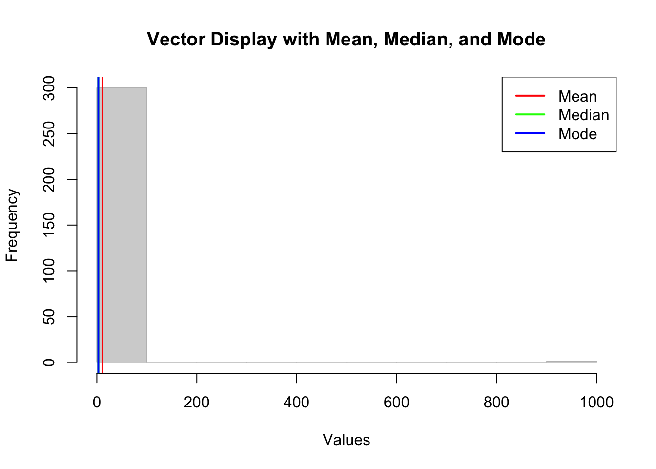
It’s clear that we have an outlier in our dataset which is having an impact on the mean, but not on the median or mode.
Reflect: What action do we need to take?
The range and standard deviation provide insights into the variability or spread of the data, indicating how much the data values diverge from the average.
I’m going to create another sample_vector which we will test for variability. I’ve deliberately created a vector that has a lot of values at the lower end, and fewer at the higher end.
First we’ll calculate and print the statistics using the psych package, and by using base R.
# Create a new sample vector
sample_vector <- c(rep(1, 50), rep(2, 25), rep(3, 20), rep(4, 5), 5)

# Method One - using the 'psych' package

library(psych)

summary_data <- describe(sample_vector)
print(summary_data)
vars n mean sd median trimmed mad min max range skew kurtosis se
X1 1 101 1.83 0.98 2 1.7 1.48 1 5 4 0.9 -0.08 0.1# Method Two - using base R
# Calculate and print the range of the vector
range_value <- range(sample_vector)
print(paste("Range: [", range_value[1], ",", range_value[2], "]", sep=""))[1] "Range: [1,5]"# Calculate and print the standard deviation
print(paste("Standard Deviation:", round(sd(sample_vector), 2)))[1] "Standard Deviation: 0.98"We can also visualise this in a couple of different ways:
# Calculate range and standard deviation
range_values <- range(sample_vector)
sd_value <- sd(sample_vector)

# Create a basic plot
plot(sample_vector, main = "Vector with Range and Standard Deviation",
     xlab = "Index", ylab = "Values", pch = 19, col = "blue")

# Marking the range
abline(h = range_values[1], col = "red", lwd = 2) # lower range
abline(h = range_values[2], col = "red", lwd = 2) # upper range

# Marking the standard deviation
mean_value <- mean(sample_vector)
abline(h = mean_value + sd_value, col = "green", lwd = 2, lty = 2) # mean + SD
abline(h = mean_value - sd_value, col = "green", lwd = 2, lty = 2) # mean - SD

# Add a legend
legend("bottomright", legend = c("Lower Range", "Upper Range", "Mean ± SD"),
       col = c("red", "red", "green"), lwd = 2, lty = c(1, 1, 2))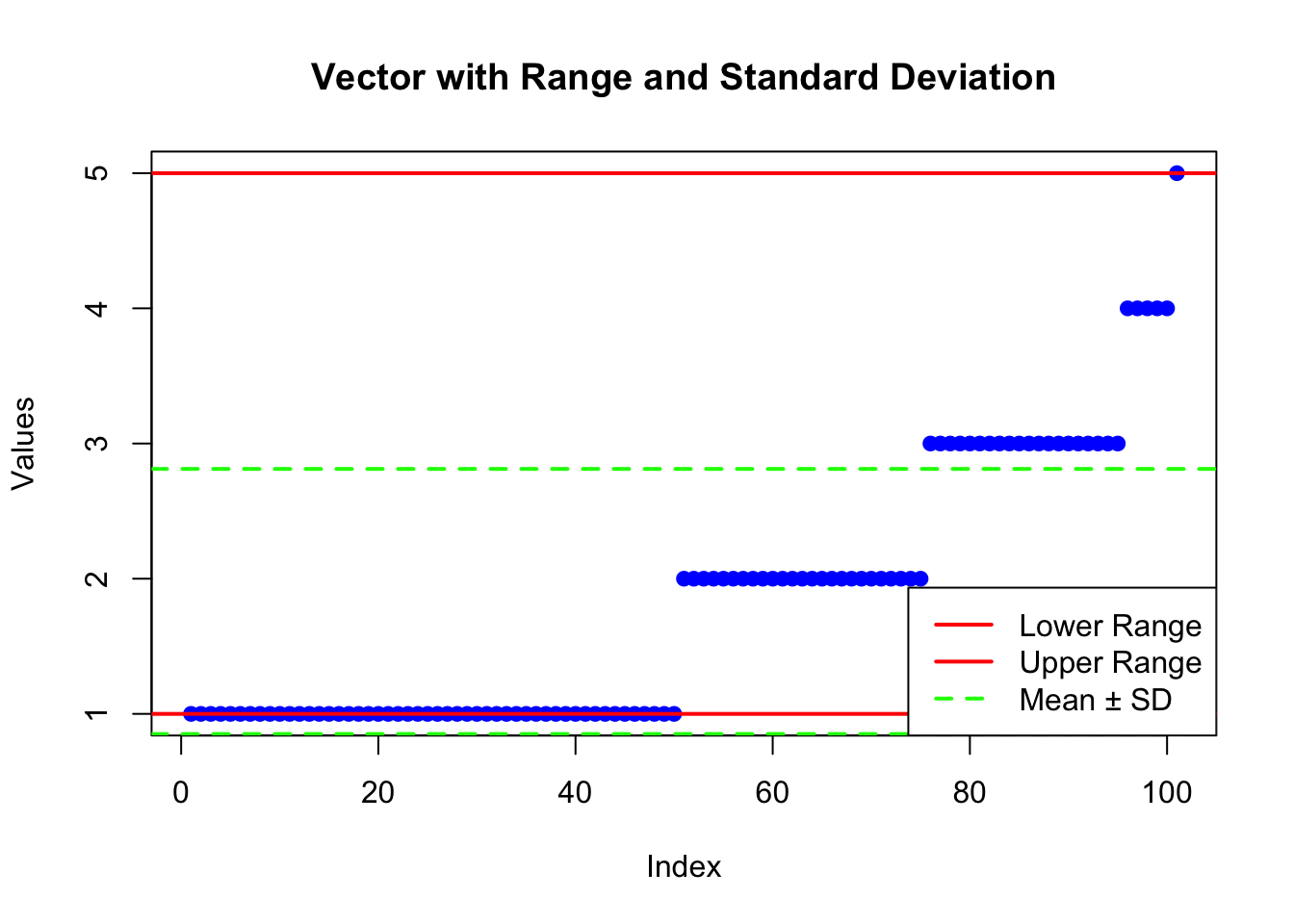
# Calculate the mean
mean_value <- mean(sample_vector)

# Create a density plot
plot(density(sample_vector), main = "Density Plot with Mean",
     xlab = "Values", ylab = "Density", col = "blue", lwd = 2)

# Marking the mean
abline(v = mean_value, col = "red", lwd = 2)

# Add a legend
legend("topright", legend = c("Mean"),
       col = c("red"), lwd = 2)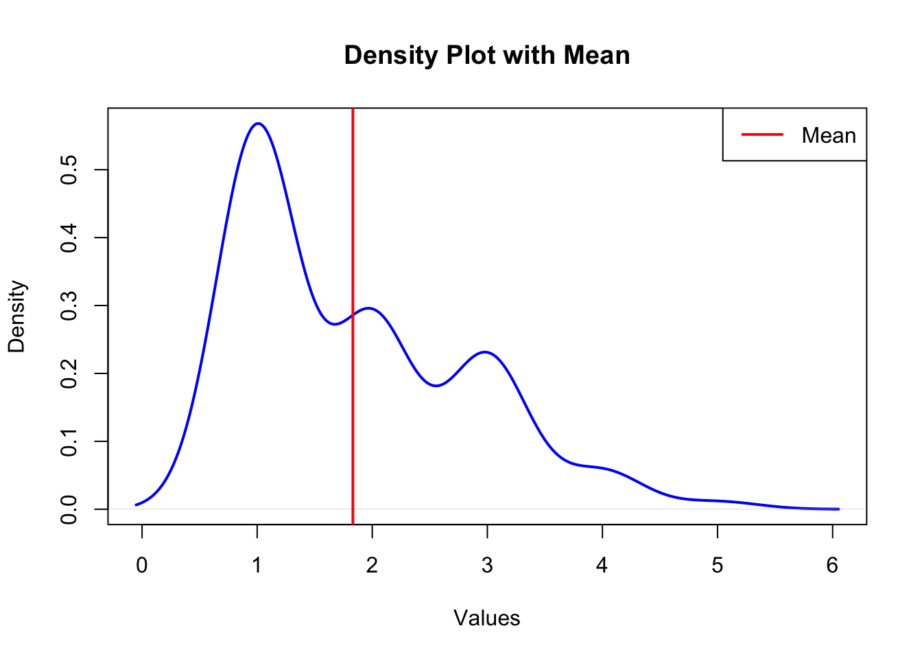
Understanding the distribution of data - whether it is skewed or symmetrical - can also be derived from descriptive measures.
As noted in the previous tutorial, there are three types of skewness.
A negatively-skewed (left-tailed) distribution looks like this:
library(ggplot2)
Attaching package: 'ggplot2'The following objects are masked from 'package:psych':
%+%, alpha# Negatively-skewed vector: More higher values and a tail on the left side.
neg_skewed_vector <- c(rep(1, 5), rep(2, 20), rep(3, 25), rep(4, 50))
# Plot the vector
ggplot(data.frame(value=neg_skewed_vector), aes(value)) +
geom_histogram(binwidth=1, fill="blue", color="black", alpha=0.7) +
labs(title="Negatively-Skewed Vector", x="Value", y="Frequency")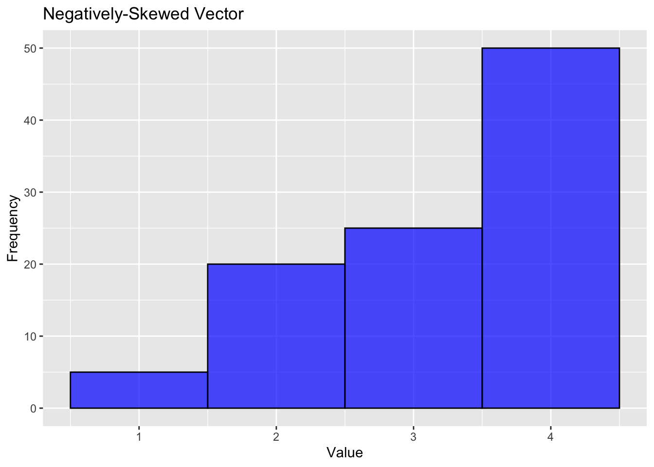
A positively-skewed (right-tailed) distribution looks like this:
# Positively-skewed vector: More lower values and a tail on the right side.
pos_skewed_vector <- c(rep(1, 50), rep(2, 25), rep(3, 20), rep(4, 5))

# Plot the vector
ggplot(data.frame(value=pos_skewed_vector), aes(value)) +
  geom_histogram(binwidth=1, fill="red", color="black", alpha=0.7) +
  labs(title="Positively-Skewed Vector", x="Value", y="Frequency")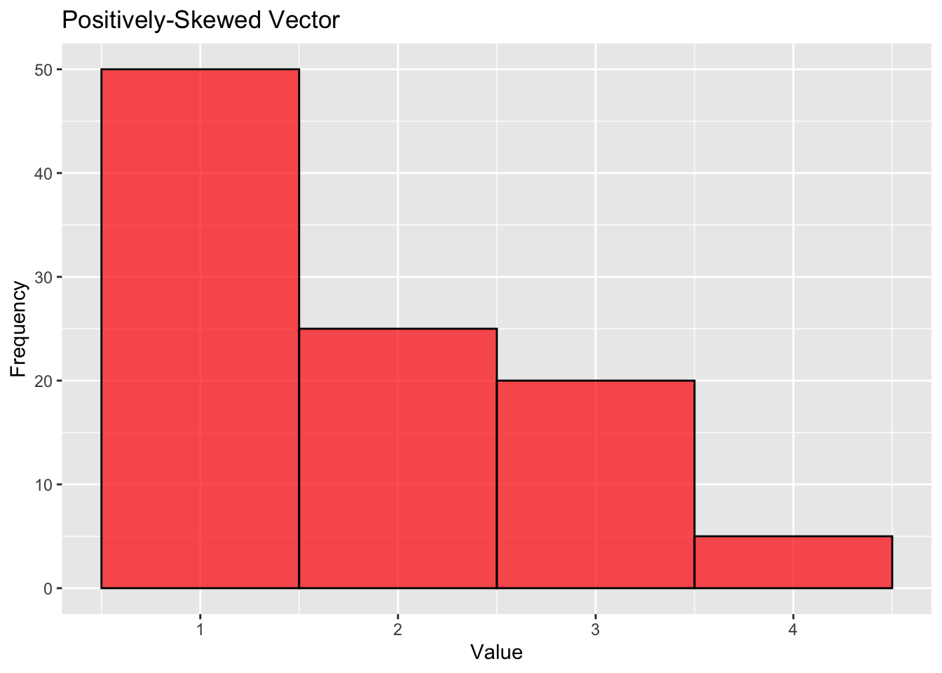
If the data is symmetric, it will look something like this:
# Symmetrical vector: Equal distribution on both sides of the central value.
symmetrical_vector <- c(rep(1, 18), rep(2, 24), rep(3, 30), rep(4, 25), rep(5,19))

# Plot the vector
ggplot(data.frame(value=symmetrical_vector), aes(value)) +
  geom_histogram(binwidth=1, fill="green", color="black", alpha=0.7) +
  labs(title="Symmetrical Vector", x="Value", y="Frequency")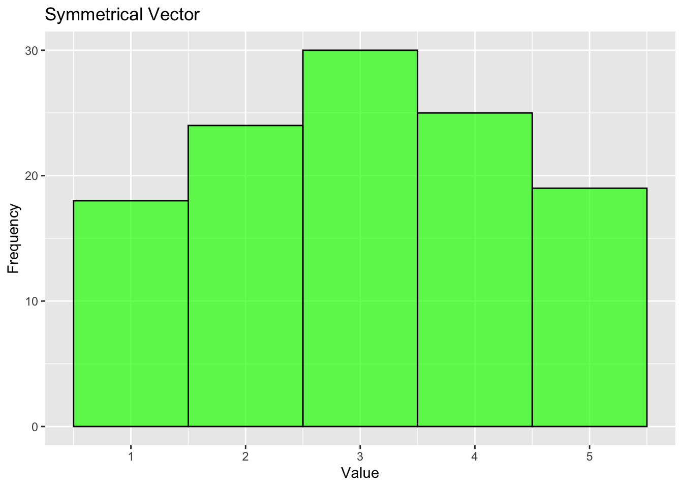
Returning to our vector, we can check the skewness as follows:
# load the e1071 package

library(e1071)

# Calculate the skewness
skew_value <- skewness(sample_vector)

# Print and describe the skewness as output in the console
print(paste("Skewness:", round(skew_value, 2)))
[1] "Skewness: 0.9"if (skew_value > 0) {
print("The distribution is positively skewed (right-tailed).")
} else if (skew_value < 0) {
print("The distribution is negatively skewed (left-tailed).")
} else {
print("The distribution is approximately symmetric.")
}[1] "The distribution is positively skewed (right-tailed)."# Plot the distribution of the vector
ggplot(data.frame(value=sample_vector), aes(value)) +
geom_histogram(binwidth=1, fill="green", color="black", alpha=0.7) +
labs(title="Sample Vector - Positively Skewed with more values to the left", x="Value", y="Frequency")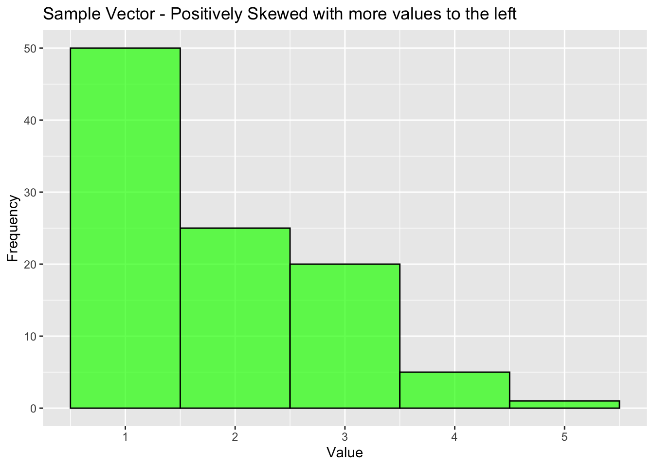
Note: The simplest way of visualising range is with a stem-and-leaf plot:
#| code-fold: true
#| code-summary: Show code for stem-and-leaf plot

# Create a stem-and-leaf plot
stem(pos_skewed_vector)
  The decimal point is at the |

  1 | 00000000000000000000000000000000000000000000000000
  1 |
  2 | 0000000000000000000000000
  2 |
  3 | 00000000000000000000
  3 |
4 | 00000Imagine you’re trying to figure out the average height of all the students in the university. It’s not practical to measure every single student, so you measure 30 students at random as they walk up Montrose Street.
Based on this smaller group, you try to make a good guess about the average height of all the students in the university
A confidence interval is like saying, “I’m pretty sure the average height of all the students is between this height and that height.” For example, you might say you’re confident the average height is between 5 feet 2 inches and 5 feet 6 inches.
The “confidence” part is like how sure you are about this range. Usually, we use a 95% confidence level. This means if you were to measure 30 students many, many times, about 95 times out of 100, the true average height of all the students would fall within your guessed range.
So, a confidence interval gives you a range where you expect the true average (or other statistic) to be, based on your smaller group, and it tells you how confident you can be about this range.
# We create a function to calculate the confidence interval of a numeric vector

calculate_confidence_interval <- function(data, confidence_level = 0.95) {
  # Check if the data is a numeric vector
  if (!is.numeric(data)) {
    stop("Data must be a numeric vector.")
  }

  # Use t.test to calculate the confidence interval
  test_result <- t.test(data, conf.level = confidence_level)

  # Extract the confidence interval
  ci <- test_result$conf.int

  # Return the confidence interval
  return(ci)
}

# Example usage
data_vector <- c(12, 15, 14, 16, 15, 14, 16, 15, 14, 15)
ci <- calculate_confidence_interval(data_vector)
print(ci)
[1] 13.76032 15.43968
attr(,"conf.level")
[1] 0.95Bar charts and histograms are useful for visualising the distribution of categorical or continuous data, and for identifying common patterns or outliers.
Bar charts are used to display the distribution of categorical data, while histograms are used to display the distribution of continuous data.
# We create some categorical data
teams <- c("Liverpool", "Man City", "Chelsea", "Brighton", "West Ham")
goals_for <- c(34, 45, 21, 15, 10)

# And some continuous data
goals <- rnorm(200, mean=30, sd=6)  # Simulated goals

# Bar chart for categorical data
bar_chart <- ggplot(data.frame(teams=teams, goals_for=goals_for), aes(x=teams, y=goals_for)) +
  geom_bar(stat="identity", fill="coral", color="black", width=0.7) +
  labs(title="Bar Chart for Categorical Data (goals for)", x="Team", y="Goals For") +
  theme_minimal()

print(bar_chart)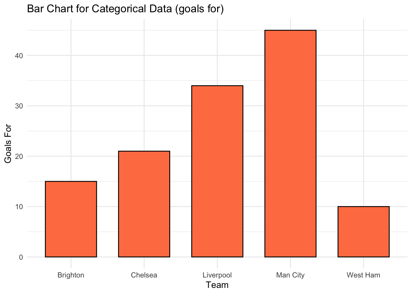
# Histogram for continuous data
histogram_plot <- ggplot(data.frame(goals=goals), aes(goals)) +
  geom_histogram(binwidth=5, fill="skyblue", color="black", alpha=0.7) +
  labs(title="Histogram for Continuous Data", x="Goals", y="Frequency") +
  theme_minimal()

print(histogram_plot)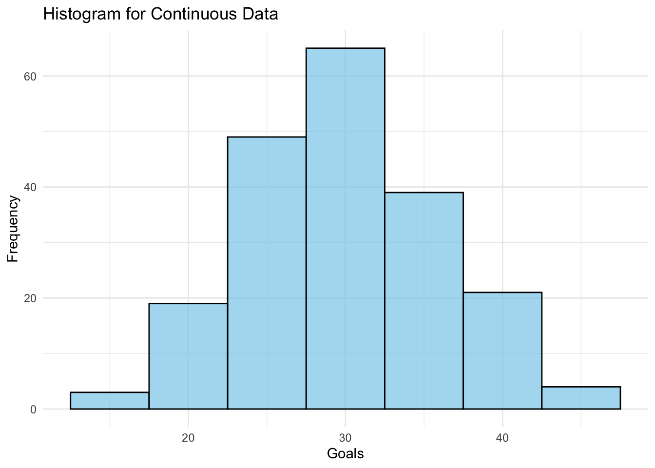
Box plots highlight the spread and the central tendency of data, and identify potential outliers.
They are very useful plots to explore your data.
# Load necessary libraries
library(dplyr)
Attaching package: 'dplyr'The following objects are masked from 'package:stats':
filter, lagThe following objects are masked from 'package:base':
intersect, setdiff, setequal, union# Set seed for reproducibility
set.seed(123)
# Generate dummy dataset
dummy_data <- data.frame(
player_id = sample(c("Player 1", "Player 2", "Player 3"), 1000, replace = TRUE),
distance_covered = runif(1000, min = 1, max = 100)
)
# View the first few rows of the dataset
head(dummy_data) player_id distance_covered
1 Player 3 36.353535
2 Player 3 97.561136
3 Player 3 39.053474
4 Player 2 49.378680
5 Player 3 49.586847
6 Player 2 2.213208# Create a boxplot
boxplot <- ggplot(dummy_data, aes(x = player_id, y = distance_covered)) +
geom_boxplot() +
labs(title = "Boxplot of Distance Covered Grouped by Player",
x = "Player",
y = "Distance (m)")
# Print the boxplot
print(boxplot)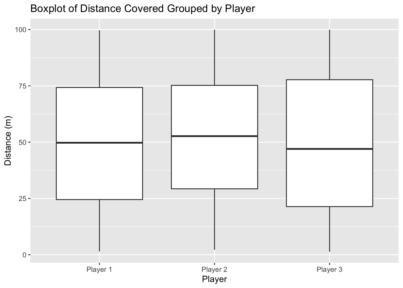
Pie charts are effective for displaying the proportions of different categories within a whole.
library(ggplot2)

# Calculate proportions for each category level
category_counts <- dummy_data %>%
  group_by(player_id) %>%
  summarise(Count = n()) %>%
  mutate(Proportion = Count / sum(Count))

# Create a pie chart
pie_chart <- ggplot(category_counts, aes(x = "", y = Proportion, fill = player_id)) +
  geom_bar(stat = "identity", width = 1) +
  coord_polar(theta = "y") +
  labs(title = "Pie Chart of Category Levels",
       fill = "Category")

# Print the pie chart
print(pie_chart)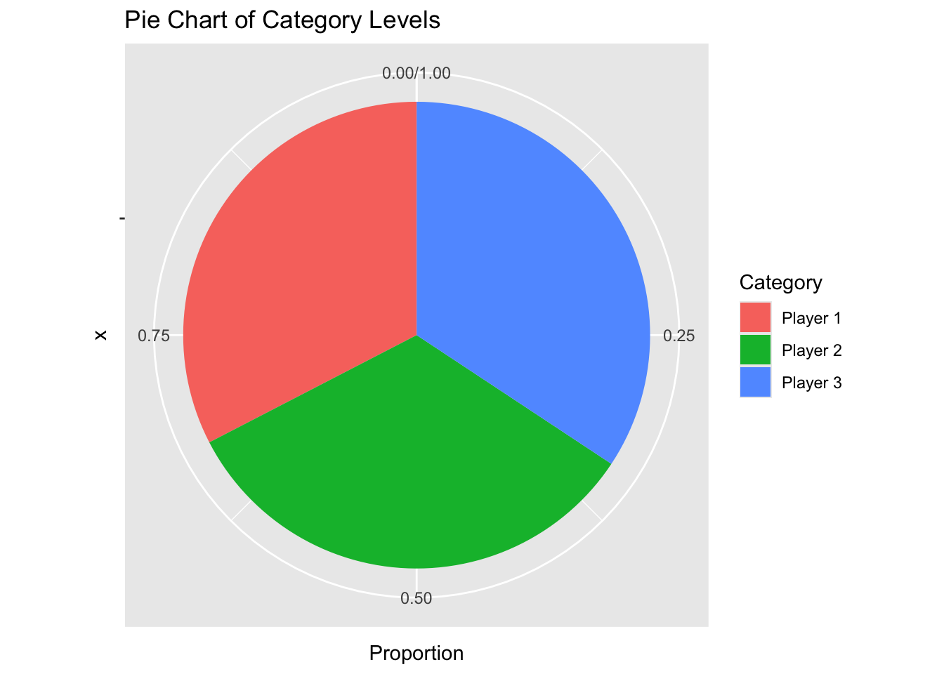
Dealing with missing data and outliers are a key challenge in any data analytics task. We need to make sure our results are not influenced by values that are ‘wrong’ (thought sadly, many analysts don’t pay too much attention to this question).
First, we’ll create vector that has some missing data:
# Set seed for reproducibility
set.seed(123)

# Generate a vector with 50 random observations from a normal distribution
observations <- rnorm(50, mean = 10, sd = 5)

# Randomly assign missing values to 10% of the observations
missing_indices <- sample(1:50, 5)
observations[missing_indices] <- NA

# Print the vector with missing values
print(observations)
[1] 7.1976218 8.8491126 17.7935416 10.3525420 10.6464387 18.5753249
[7] 12.3045810 3.6746938 6.5657357 7.7716901 16.1204090 11.7990691
[13] 12.0038573 10.5534136 7.2207943 18.9345657 12.4892524 0.1669142
[19] 13.5067795 7.6360430 4.6608815 NA 4.8699778 6.3555439
[25] NA 1.5665334 14.1889352 10.7668656 4.3093153 16.2690746
[31] 12.1323211 NA 14.4756283 14.3906674 14.1079054 13.4432013
[37] 12.7695883 9.6904414 8.4701867 8.0976450 6.5264651 8.9604136
[43] 3.6730182 20.8447798 16.0398100 NA 7.9855758 7.6667232
[49] 13.8998256 NAWe can see that there are a number of missing (NA) values in our vector.
There are two main strategies to deal with this. The first is to **remove* any observations that have missing data.
# Removing observations with missing values
clean_observations <- observations[!is.na(observations)]

# Printing the cleaned observations
print(clean_observations)
[1] 7.1976218 8.8491126 17.7935416 10.3525420 10.6464387 18.5753249
[7] 12.3045810 3.6746938 6.5657357 7.7716901 16.1204090 11.7990691
[13] 12.0038573 10.5534136 7.2207943 18.9345657 12.4892524 0.1669142
[19] 13.5067795 7.6360430 4.6608815 4.8699778 6.3555439 1.5665334
[25] 14.1889352 10.7668656 4.3093153 16.2690746 12.1323211 14.4756283
[31] 14.3906674 14.1079054 13.4432013 12.7695883 9.6904414 8.4701867
[37] 8.0976450 6.5264651 8.9604136 3.6730182 20.8447798 16.0398100
[43] 7.9855758 7.6667232 13.8998256The danger with this approach is that it might lead to the removal of lots of observations, especially if you run it on a dataframe that has many variables with missing data.
The second is to impute a new (‘reasonable’) value and replace the missing value with that value.
# We can imputing missing values with a specific value, for example, 0
imputed_observations_01 <- ifelse(is.na(observations), 0, observations)

# Printing the imputed observations
print(imputed_observations_01)
[1] 7.1976218 8.8491126 17.7935416 10.3525420 10.6464387 18.5753249
[7] 12.3045810 3.6746938 6.5657357 7.7716901 16.1204090 11.7990691
[13] 12.0038573 10.5534136 7.2207943 18.9345657 12.4892524 0.1669142
[19] 13.5067795 7.6360430 4.6608815 0.0000000 4.8699778 6.3555439
[25] 0.0000000 1.5665334 14.1889352 10.7668656 4.3093153 16.2690746
[31] 12.1323211 0.0000000 14.4756283 14.3906674 14.1079054 13.4432013
[37] 12.7695883 9.6904414 8.4701867 8.0976450 6.5264651 8.9604136
[43] 3.6730182 20.8447798 16.0398100 0.0000000 7.9855758 7.6667232
[49] 13.8998256 0.0000000# Often, we might want to use the mean of the vector.
# Calculating the mean of the non-missing values
mean_value <- mean(observations, na.rm = TRUE)
print(mean_value)[1] 10.45164# Imputing missing values with the calculated mean
imputed_observations_02 <- ifelse(is.na(observations), mean_value, observations)
# Printing the imputed observations
print(imputed_observations_02) [1] 7.1976218 8.8491126 17.7935416 10.3525420 10.6464387 18.5753249
[7] 12.3045810 3.6746938 6.5657357 7.7716901 16.1204090 11.7990691
[13] 12.0038573 10.5534136 7.2207943 18.9345657 12.4892524 0.1669142
[19] 13.5067795 7.6360430 4.6608815 10.4516379 4.8699778 6.3555439
[25] 10.4516379 1.5665334 14.1889352 10.7668656 4.3093153 16.2690746
[31] 12.1323211 10.4516379 14.4756283 14.3906674 14.1079054 13.4432013
[37] 12.7695883 9.6904414 8.4701867 8.0976450 6.5264651 8.9604136
[43] 3.6730182 20.8447798 16.0398100 10.4516379 7.9855758 7.6667232
[49] 13.8998256 10.4516379The previous code works on a single vector. You may want to address missing data in multiple vectors at the same time (e.g. as part of a data frame).
The following code allows you to remove observations where there is a missing value in ANY variable/column.
# Creating a dataframe with two variables containing missing values
data <- data.frame(
  variable1 = c(1, NA, 3, 4, NA, 6),
  variable2 = c(NA, 2, NA, 4, 5, NA)
)

# Printing the original dataframe
print("Original Dataframe:")
[1] "Original Dataframe:"print(data) variable1 variable2
1 1 NA
2 NA 2
3 3 NA
4 4 4
5 NA 5
6 6 NA# Removing observations with a missing value in EITHER variable
clean_data <- na.omit(data)
# Printing the cleaned dataframe
print("Cleaned Dataframe:")[1] "Cleaned Dataframe:"print(clean_data) variable1 variable2
4 4 4As before, you might want to impute a value for a missing value, rather than delete the entire observation.
The following code imputes the mean of the column and uses it to replace missing values in that column.
# Loading the dplyr package for easier data manipulation
library(dplyr)

# Creating a dataframe with two variables containing missing values
data <- data.frame(
  variable1 = c(1, NA, 3, 4, NA, 6),
  variable2 = c(NA, 2, NA, 4, 5, NA)
)

# Printing the original dataframe
print("Original Dataframe:")
[1] "Original Dataframe:"print(data) variable1 variable2
1 1 NA
2 NA 2
3 3 NA
4 4 4
5 NA 5
6 6 NA# Function to replace NA with the mean of the column
replace_na_with_mean <- function(x) {
x[is.na(x)] <- mean(x, na.rm = TRUE)
return(x)
}
# Applying the function to each column using `across`
imputed_data <- data %>% mutate(across(everything(), replace_na_with_mean))
# Printing the dataframe with imputed values
print("Dataframe with Imputed Values:")[1] "Dataframe with Imputed Values:"print(imputed_data) variable1 variable2
1 1.0 3.666667
2 3.5 2.000000
3 3.0 3.666667
4 4.0 4.000000
5 3.5 5.000000
6 6.0 3.666667As with missing data, there are two main approaches to dealing with observations (rows) where outliers are present.
The first is to simply remove
# Remove outliers based on Z-scores

# Generate a synthetic dataset
set.seed(123) # for reproducibility
data <- data.frame(value = rnorm(100, mean = 50, sd = 10)) # synthetic normal data

# Function to calculate Z-scores
calculate_z_score <- function(x) {
  (x - mean(x)) / sd(x)
}

# Apply the function to calculate Z-scores for the dataset
data$z_score <- calculate_z_score(data$value)

# Define threshold for outliers
lower_bound <- -3
upper_bound <- 3

# Remove outliers
cleaned_data <- data[data$z_score > lower_bound & data$z_score < upper_bound, ]

# View the cleaned data
print(cleaned_data)
value z_score
1 44.39524 -0.71304802
2 47.69823 -0.35120270
3 65.58708 1.60854170
4 50.70508 -0.02179795
5 51.29288 0.04259548
6 67.15065 1.77983218
7 54.60916 0.40589817
8 37.34939 -1.48492941
9 43.13147 -0.85149566
10 45.54338 -0.58726835
11 62.24082 1.24195461
12 53.59814 0.29513939
13 54.00771 0.34000892
14 51.10683 0.02221347
15 44.44159 -0.70797086
16 67.86913 1.85854263
17 54.97850 0.44636008
18 30.33383 -2.25349176
19 57.01356 0.66930255
20 45.27209 -0.61698896
21 39.32176 -1.26885349
22 47.82025 -0.33783464
23 39.73996 -1.22304003
24 42.71109 -0.89754917
25 43.74961 -0.78377819
26 33.13307 -1.94683206
27 58.37787 0.81876439
28 51.53373 0.06898128
29 38.61863 -1.34588242
30 62.53815 1.27452758
31 54.26464 0.36815564
32 47.04929 -0.42229479
33 58.95126 0.88157948
34 58.78133 0.86296437
35 58.21581 0.80101058
36 56.88640 0.65537241
37 55.53918 0.50778230
38 49.38088 -0.16686565
39 46.94037 -0.43422620
40 46.19529 -0.51585092
41 43.05293 -0.86009994
42 47.92083 -0.32681639
43 37.34604 -1.48529653
44 71.68956 2.27707482
45 62.07962 1.22429519
46 38.76891 -1.32941869
47 45.97115 -0.54040552
48 45.33345 -0.61026684
49 57.79965 0.75541982
50 49.16631 -0.19037243
51 52.53319 0.17847258
52 49.71453 -0.13031397
53 49.57130 -0.14600575
54 63.68602 1.40027842
55 47.74229 -0.34637532
56 65.16471 1.56226982
57 34.51247 -1.79571669
58 55.84614 0.54141021
59 51.23854 0.03664303
60 52.15942 0.13752572
61 53.79639 0.31685861
62 44.97677 -0.64934164
63 46.66793 -0.46407310
64 39.81425 -1.21490140
65 39.28209 -1.27319995
66 53.03529 0.23347834
67 54.48210 0.39197814
68 50.53004 -0.04097396
69 59.22267 0.91131364
70 70.50085 2.14685001
71 45.08969 -0.63697081
72 26.90831 -2.62876100
73 60.05739 1.00275711
74 42.90799 -0.87597805
75 43.11991 -0.85276181
76 60.25571 1.02448422
77 47.15227 -0.41101270
78 37.79282 -1.43635058
79 51.81303 0.09957931
80 48.61109 -0.25119772
81 50.05764 -0.09272595
82 53.85280 0.32303830
83 46.29340 -0.50510289
84 56.44377 0.60688103
85 47.79513 -0.34058618
86 53.31782 0.26443017
87 60.96839 1.10255872
88 54.35181 0.37770550
89 46.74068 -0.45610238
90 61.48808 1.15949090
91 59.93504 0.98935390
92 55.48397 0.50173432
93 52.38732 0.16249260
94 43.72094 -0.78691881
95 63.60652 1.39156928
96 43.99740 -0.75663177
97 71.87333 2.29720706
98 65.32611 1.57995139
99 47.64300 -0.35725306
100 39.73579 -1.22349625Again, this runs the risk that we remove a significant amount of observations. An alternative approach, as for missing data, is to impute a value that is reasonable and replace the outlier with that value:
# Generate a synthetic dataset

set.seed(123) # for reproducibility
data <- data.frame(value = rnorm(100, mean = 50, sd = 10)) # synthetic normal data

# Function to calculate Z-scores
calculate_z_score <- function(x) {
  (x - mean(x)) / sd(x)
}

# Apply the function to calculate Z-scores for the dataset
data$z_score <- calculate_z_score(data$value)

# Define threshold for outliers
lower_bound <- -3
upper_bound <- 3

# Impute outliers using the mean
data$value[data$z_score < lower_bound] <- mean(data$value) - 3 * sd(data$value)
data$value[data$z_score > upper_bound] <- mean(data$value) + 3 * sd(data$value)

# Remove the z_score column if no longer needed
data$z_score <- NULL

# View the modified data
print(data)
value
1 44.39524
2 47.69823
3 65.58708
4 50.70508
5 51.29288
6 67.15065
7 54.60916
8 37.34939
9 43.13147
10 45.54338
11 62.24082
12 53.59814
13 54.00771
14 51.10683
15 44.44159
16 67.86913
17 54.97850
18 30.33383
19 57.01356
20 45.27209
21 39.32176
22 47.82025
23 39.73996
24 42.71109
25 43.74961
26 33.13307
27 58.37787
28 51.53373
29 38.61863
30 62.53815
31 54.26464
32 47.04929
33 58.95126
34 58.78133
35 58.21581
36 56.88640
37 55.53918
38 49.38088
39 46.94037
40 46.19529
41 43.05293
42 47.92083
43 37.34604
44 71.68956
45 62.07962
46 38.76891
47 45.97115
48 45.33345
49 57.79965
50 49.16631
51 52.53319
52 49.71453
53 49.57130
54 63.68602
55 47.74229
56 65.16471
57 34.51247
58 55.84614
59 51.23854
60 52.15942
61 53.79639
62 44.97677
63 46.66793
64 39.81425
65 39.28209
66 53.03529
67 54.48210
68 50.53004
69 59.22267
70 70.50085
71 45.08969
72 26.90831
73 60.05739
74 42.90799
75 43.11991
76 60.25571
77 47.15227
78 37.79282
79 51.81303
80 48.61109
81 50.05764
82 53.85280
83 46.29340
84 56.44377
85 47.79513
86 53.31782
87 60.96839
88 54.35181
89 46.74068
90 61.48808
91 59.93504
92 55.48397
93 52.38732
94 43.72094
95 63.60652
96 43.99740
97 71.87333
98 65.32611
99 47.64300
100 39.73579First, download the dataset here:
url <- "https://www.dropbox.com/scl/fi/fmqfeq6ivdrvnr4hy79ny/prac_14_dataset.csv?rlkey=spz5e5uq1b8if2eptvstxo7xj&dl=1"
df <- read.csv(url)
rm(url)
Apply the following steps to the dataframe df.
One of the vectors in the dataframe df contains a significant number of missing values.
From what you have learned so far/discussing the situation with others/engaging in some further reading or research, identify the vector with missing data, and deal with any missing data in the dataframe in the following ways:
One of the vectors in the dataframe df contains a significant number of outliers.
From what you have learned so far, by discussing the situation with others, or by engaging in some further reading/research, identify potential outliers and deal with them in the following ways:
For each variable in the dataframe that is suitable for this kind of analysis, calculate the mean, mode and median.
One of the variables in the dataframe has a very different mean, mode, and median. Which variable does this apply to?
For any variables that are not suitable for this kind of analysis, what other measure of ‘central tendency’ (if any) would it be useful to calculate and report.
For each variable in the dataframe that is suitable for this kind of analysis, calculate the measures of variability that were discussed above.
For any variables that are not suitable for this kind of analysis, what other measure of variability (if any) would it be useful to calculate and report.
One variable in the dataframe has a clear negative skew. Which variable or variables does this apply to?
Another variable in the dataframe has a clear positive skew. Again, which variable or variables does this description apply to?
#Var1 has a bimodal distribution, which will result in different mean, mode, and median.
#Var2 is generated from a chi-squared distribution, which is skewed to the right (negative skewness).
#Var3 is generated from an exponential distribution, which is skewed to the left (positive skewness).
#Group is a factor variable with three levels.
#Var5 has a lot of missing data, with approximately 30% NA values.
#Var6 has a large number of outliers, with 10% of the data being extreme values.